Overview of GANs - Part I

Background

What is meant by generative? At a high level, a generative model means you have mapped the probability distribution of the data itself. In the case of images, that means you have a probability for every possible combination of pixel values. This also means you can generate new data points by sampling from this distribution (i.e. choosing combinations with large probability). If you’re in a computer vision domain, that means your model can create new images from scratch. Here, for example, is a generated face.

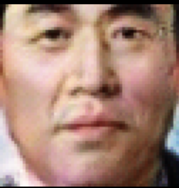
In case this hasn’t totally sunk in yet: this is not a real person, it’s a computer-invented face. A GAN can do this because it was given a lot of images of faces to learn from and that resulted in a probability distribution. This image is one point taken from that distribution. With generative models you can create new stuff that didn’t previously exist. Audio, text, images…etc. Very, very cool stuff.

The Original GAN

The original paper by Ian Goodfellow, et al. outlined the basic approach, built the theoretical foundation and gave some example benchmarks.

GANs did not invent generative models, but rather provided an interesting and convenient way to learn them. They are called “adversarial” because the problem is structured such that two entities are competing against one another, and both of those entities are machine learning models.

This is best explained with an example. Let’s say you want to build a face-image generator. You start by feeding in a bunch of random numbers to a system, and it adds them and multiplies them and applies fancy functions. At the end of this, it outputs a brightness value for each pixel. This is your generative model — you give it noise and it generates data. Now, let’s say you do this 10 different times and get 10 different fake images.

Next, you grab 10 images of real faces. Then, you feed both the fake and real images into a different model called the Discriminator. Its job is to output a number for each input image which tells you the probability that the image is real. In the beginning, the generated samples are just noise, so you might think this would be easy, but the Discriminator is just as bad because it has not learned anything yet either.

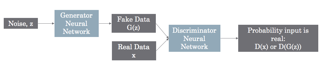
For each mistake on a fake image, the Discriminator gets penalized and the Generator gets rewarded. The Discriminator is also penalized or rewarded based on classifying the real images correctly. This is why they’re called adversarial — the Discriminator’s loss is the Generator’s gain. Over time, the competition leads to mutual improvement.

Finally, the word “networks” is used because the authors use a neural network for modeling both the Generator and Discriminator. This is awesome because it provides an easy framework for using the penalties/rewards to tweak the network parameters such that they learn: the familiar back-propagation.

Theoretical Foundations

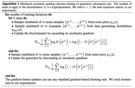
I won’t recreate all the gory details of the paper, but it’s worth mentioning they show both:

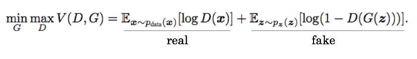
• The optimization objective \( V(D,G) \) results in the Generator probability distribution exactly matching the true probability distribution. This means your fake examples are indistinguishable from real examples.

• The authors’ gradient ascent/descent training algorithm converges to this optimum. So you not only know what you need to do, but how to do it.

To build intuition, in the above optimization objective \( V(D,G) \), the term \( D(x) \) is the Discriminator’s answer to the question: What’s the probability that input \( x \) is from the real data set? If you plug \( G(z) \) in to this function, it’s the Discriminator’s guess when you give it fake data. If you consider \( D \) and \( G \) separately you’ll see that \( G \) wants \( V(D,G) \) to be small and \( D \) wants this to be large. This motivates the gradient ascent/descent technique in the algorithm. [The \( E \) means “expectation”, which is just an average. The subscript shows you which probability distribution you’re averaging over, either the real data or the noise that the Generator turns into fake images].

However, their provided proof doesn’t directly apply since we’re indirectly optimizing these probability distributions by optimizing parameters of a neural networks, but it’s nice to know that the foundation has theoretical guarantees.

Results

It’s worth noting that it’s difficult to quantify the quality of fake data. How does one judge the improvement in fake-face generation? That aside, they have state of the art performance when it comes to generating realistic images, which is driving a lot of the buzz. Images generally look less blurry than alternative approaches.

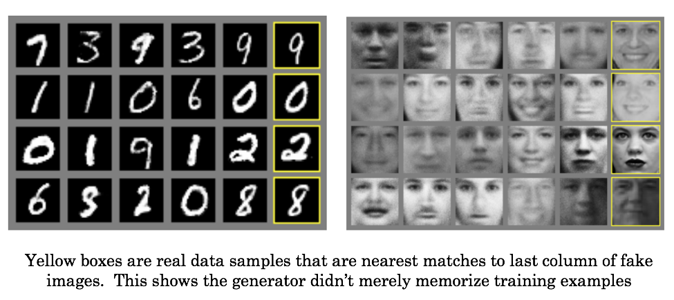
Although advancements have been made since the original paper (which will be covered in Part II), here are some examples from it:

Problems

The biggest problems with the original GAN implementation are:

• Training difficultly. Sometimes the models will never learn anything or converge to a local minima.
• “Mode collapse”, which is when the Generator essentially outputs the same thing over and over.

These problems are addressed by refinements to the architecture and will be presented in future posts.

Conclusion

Ultimately, this framework allows us to use the normally supervised learning approach of neural networks in an unsupervised way. This is because our labels are trivial to generate since we know which data came from the training set and which data were generated. It’s worth noting that in the above images of hand-written digits, the digit labels themselves were not used during training. Despite this, the Generator and Discriminator are both able to learn useful representations of the data, as demonstrated by the Generator’s capability of mimicking the data.

In Part II we’ll discuss how to fix many of the training problems as well as make substantial improvements in realistic image generation.