
Introduction
In the march toward Machine Learning ubiquity, AutoML is emerging as an important mechanism for making ML accessible to those without deep expertise in the field. Simply put, the aspiration of AutoML is to allow a “push-button” experience, where the user provides data, pushes a button, and gets an ML model out the other end.
In the case of neural networks, determining the network structure is an important challenge–e.g. how many layers, how many nodes per layer, how are the layers connected together? The typical advice is to just choose as large a model as you can get away with from the perspective of hardware capabilities and speed, and then use standard practices to prevent overfitting.
The AdaNet paper from Google Research proposes a new algorithm that allows us to learn the optimal network structure. The theory they develop and apply in the paper was quite different from what I am used to reading, and I learned a valuable perspective by working through it. I'll try to present my understanding of it here in a more accessible format with the hope that others might enjoy and benefit from their perspective.
Framing the Problem
Generalization Error
The primary goal of supervised ML is to learn a model that provides good predictions on new data, i.e. minimizes the Generalization Error. The typical approach to this is to first optimize the model parameters to learn to make good predictions on training data. However, it's well-known that using Maximum Likelihood techniques alone to learn model parameters result in a model that performs well on the training data, but may not generalize well to new data since it also fits to noise in the training data. As such, a variety of techniques have been developed that in one way or another attempt to constrain the complexity of the model (e.g. regularization, dropout, early stopping…etc) so that it stops short of fitting to the noise. The model is then developed using an iterative cycle in which the degree of overfitting is evaluated by using a holdout dataset, and then the model is re-trained using different parameters with the aim to ultimately reduce generalization error.
This paper takes a different approach. The authors develop theory that results in an equation for directly estimating the upper bound on Generalization Error. Intuitively, this equation turns out to depend on a trade-off between training data performance and model complexity. Having an explicit equation for Generalization Error (as well as an algorithm for minimizing it) gives us a recipe for making good trade-off decisions between training performance and complexity. Since the model complexity depends on the neural network structure and properties of the training data, we can learn an optimal structure of our network.
Ensembles
First, it should be noted that this paper is an extension of the techniques developed in the Deep Boosting paper by some of the same authors. Whereas that paper was in the context of ensembles of trees, this paper extends similar techniques to the world of neural networks. Fundamental to this work is treating the “ultimate model” as an ensemble of simpler “sub-models” (terms in quotes are my informal terminology, not the papers’). This means:
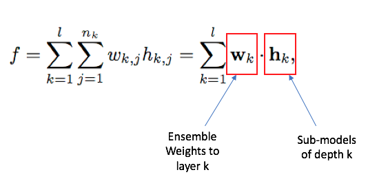
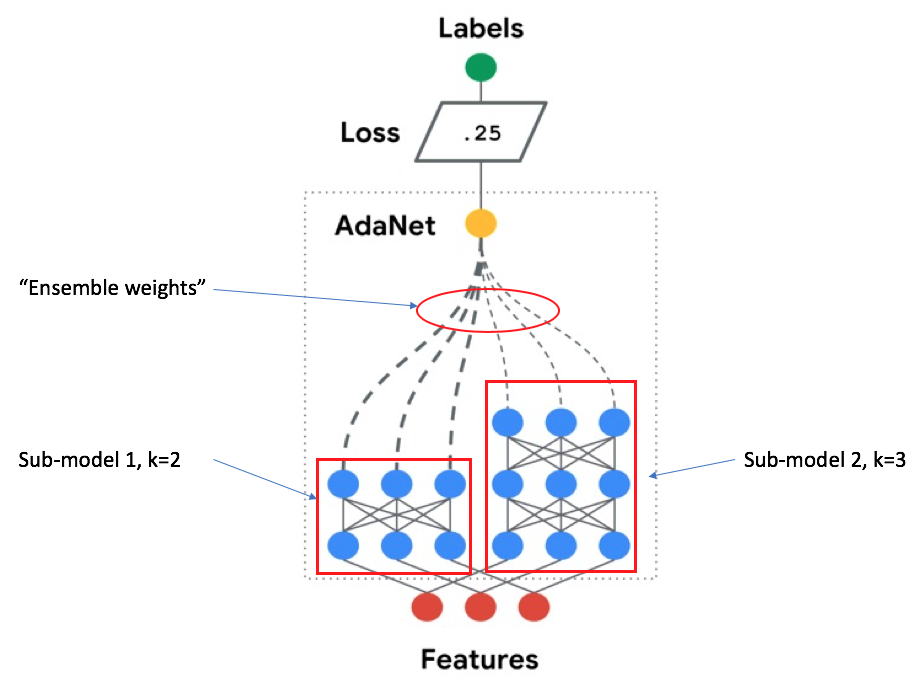
where the “ultimate model” \( f \) is a weighted sum of sub-models, with \( w \) representing the weights and \( h \) representing the sub-models. In the case of trees, the ensemble learns optimal weights for each tree's decision. In the case of neural networks, this is just another dense layer with a single output node which is connected to all the output nodes of sub-model layers. The following is an example network architecture where there are two sub-models, each with 3 output nodes per layer, but having different depths:
Theory
Calculating Generalization Error
Instead of trying to re-create the proof here, I'll just discuss the interesting aspects of the results. The equation for the upper bound on Generalization Error is as follows:


In English, this roughly says:
Generalization error <= Training Error + ensemble_weights*submodel_complexity + stuff that depends on the size of your training data and max depth of neural network.
I want to call particular attention to this part:

Generalization Error =~ ensemble weights on the sub-networks?! That's great news! This means we can:
- Improve generalization error by modifying the weights we apply to the various components in our ensemble.
- Allow complicated models (i.e. deep layers), as long as we compensate by giving them small weights.
This gives us a principled method for deciding when to include a more complicated model in our ensemble to further reduce the training error: we should do this when the decrease in training error is larger than the increase in the complexity term.
Complexity
We've so far seen how model complexity comes into the picture for estimating Generalization Error, but not how to calculate model complexity itself. In this world of research, the concept of Rademacher Complexity seems to be the standard. This was not a concept I was familiar with prior to reading the paper. My understanding is that it measures the degree to which a family of functions can fit noise. At a high level, you could imagine that some complicated deep neural network is likely to better fit a randomly generated training dataset than logistic regression. Rademacher Complexity is a formulation for quantifying this capacity.
Further, Empirical Rademacher Complexity quantifies how well a family of functions can fit noise on a particular dataset. Although I'm not 100% confident in my understanding, I think the idea is that some datasets naturally allow a model to fit more complicated functions than others. For instance, if you imagine a dataset of 100 rows of a single binary feature, your ability to use that feature to predict noise labels is limited, even with a deep neural net. However, if you had 1000s of high cardinality features, you could fit to noise labels much easier. In this way, the model complexity is dependent on the training dataset. This is a feature, not a bug, because a data-dependent complexity measure allows for an understanding that some datasets require more complicated models than others (e.g. speech recognition vs iris species classification).
The hard part is using the general definition of Rademacher Complexity to derive an upper bound for a particular family of functions. Luckily, the AdaNet paper does this for feed-forward neural networks:
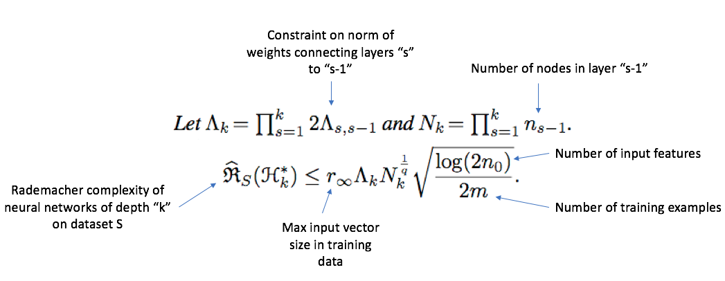
All of these terms are related to the structure of the neural network (e.g. \( \Lambda_{s, s-1} \) are constraints on the norm of connections between layers \( s \) and \( s-1 \) ) or the properties of the training dataset.
So what?
Ok, let's take a deep breath and recover from all these equations. So far, we have an equation for Generalization Error of an ensemble of neural networks. It depends on the weights of connections to sub-models, which we control, and the complexity of the layer it is connected to. The complexity of the layer is determined by the structure of the network–e.g. more/deeper layers and a larger number of nodes increase the complexity, and properties of our training dataset.
By treating this equation as a cost function and minimizing it, we can learn the optimal structure of an ensemble of neural networks in a principled way. Prior to this innovation, we just chose a network structure, and iteratively tuned parameters for in-direct complexity-penalty methods such as dropout and early stopping. Or we treated the structural parameters, like number of layers, as another hyper-parameter, and ran a lot of trials to tune everything.
But there's still something we haven't discussed: what's the recipe for generating one of these ensembles and navigating the network architecture search space?
The Actual Algorithm
There's more than one way to do this, but the authors suggest a fairly straight-forward approach:
- Train two candidate sub-networks (this has nothing to do with the ensemble)
- One with the same number of layers as was used in the previous iteration
- One with one additional layer as previous iteration.
- Once training of the sub-networks is complete, peel off the last node to expose the last hidden layer, and then plug each one into the ensemble by learning weights to connect that last layer to the ensemble's output. This is done independently for each candidate sub-network from Step 1.
- This step uses the Generalization Error equation as the cost function, which quantifies the trade-off between training error and sub-network complexity.
- Choose the candidate that led to the lowest Generalization Error for the ensemble
- Repeat from Step 1 until improvement in Generalization Error stops.
Here is an animation from the Official repo that illustrates this process:

Notice that this is an adaptive process that starts simple, and increases complexity through time. If the problem at hand requires a more complicated model, the algorithm will run for longer and grow that structure. If the model has enough complexity/capacity, generalization error bottoms out and the algorithm terminates. This is a greedy search, similar to how a decision tree chooses its split-points one-at-a-time instead of trying to jointly optimize all split-points. Generally, this might lead to sub-optimal results. However, that are standard guarantees that we still get convergence for regularized boosting if we continue to reduce our objective (see original paper for more discussion and references).
Experimental Results
The authors applied their methodology to some image classification tasks using the CIFAR-10 dataset. They compared two standard approaches for tuning neural networks: random grid search over structural + learning parameters (NN) and applying Bayesian Optimization to help search this same hyper-parameter space (NN-GP), which is the sort of HPO process that powers Amazon SageMaker.
The punch line is that AdaNet performed better. However, observe the final structures that these various approaches settled on for different image classification tasks:
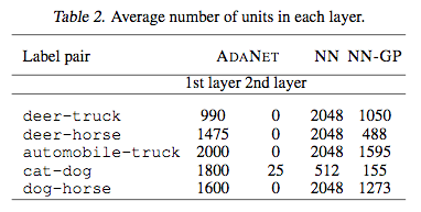
NN and NN-GP always choose one layer in these examples. This is also the case for AdaNet with the exception of differentiating between cats and dogs, which grew a 2nd layer. It matches our intuition that this would be a more complicated task than, say, differentiating between a deer and a truck. It's also interesting to note that in most cases, AdaNet grew a smaller network than the other approaches, while still beating them in performance.
Finally, the authors compared AdaNet to GP-NN on a the Criteo click prediction dataset, which is known to be a challenging classification task. (Bayesian Optimization was also applied to AdaNet's hyper-parameter search). In this case, GP-NN chose four hidden layers of 512 units each. AdaNet was able to achieve better performance using a single layer of 512 units.
Conclusion
This work takes an interesting approach in that it directly attempts to quantify/minimize an estimate of Generalization Error. Surprisingly, this turns out to be a learnable task that adapts the weights applied to sub-models of an ensemble based on training error and the sub-model complexities, which in turn depend on their structure. Paired with a simple search algorithm, this allows us to adaptively generate neural network structures to find the right level of model complexity for the problem at hand.
This approach is not free, however. We still have hyper-parameters we need to tune by using a holdout set, such as the learning rate, the starting number of nodes/layers, the strength of the complexity penalty…etc. But, this process tends to learn better performing and more efficient structures. By directly minimizing Generalization Error, we can make more principled decisions on model structure instead of e.g. choosing an unnecessarily large model and trying to tune our way out of over-fitting with indirect methods.
To try AdaNet yourself, please check out the Official repo.