Challenges of ML with PII data

Introduction

In Part 1 of this series, a case was made for why ML is a good fit for fraud systems and how it unblocks the notion of a “trust score”, which can totally change how a business manages fraud risk. The next couple posts will be written for the ML practitioners and dive deeper into some challenges of building ML fraud systems. This post will focus on the challenges of modeling with Personally Identifiable Information (PII) and consider the various trade-offs of differing strategies. This is critical in the case of Fraud ML because most of the data available is of this type, and many of the traditional techniques do not work well.

Challenges of modeling PII data

PII data are things like e-mail address, IP address, credit card number and billing address. The intent of this data is to identify individuals. From a modeling perspective, we might classify this data as high-cardinality categorical data (i.e., many distinct values). For example, there are about 4 billion IP addresses, 1 trillion possible credit card numbers, 10 billion US phone numbers and a huge number of possible e-mail addresses…etc. Almost all non-behaviorial data is PII in fraud systems, and it is therefore critical to use PII data for making decisions on new users.

How should we use PII data in models? At the end of the day, we need to convert these values into numerical representations that result in useful risk modeling. The typical trick for categorical data is one-hot encoding (OHE), which will create a new column for each possible value and put a “1” in the column corresponding to the current value, and “0"s elsewhere. For example, if our data is T-shirt size and we have the records: ["S", "M", "L", "S", "L"], then the OHE process would create three columns corresponding to the unique categories of “S”, “M” and “L” and transform the records to:

[1, 0, 0],
[0, 1, 0],
[0, 0, 1],
[1, 0, 0],
[0, 0, 1]

This will not work for PII data, however, because we would end up with billions or trillions of columns, each of which had a small number of non-zero entries.

Even if we could train a model on this data, it would not be useful. When we start making predictions on new PII data tomorrow, we would not have a corresponding OHE column since the value wasn't present during training. In our previous example, that would be like training the model on only S, M and L t-shirt sizes but then evaluating with a new “XXL” size–it would have no sensible way of making a prediction. Stepping back from the details, it is intuitive that simply learning that IP address 1 is fraud doesn't help you at all with making a prediction on IP address 2. Training a model on OHE PII data will effectively build an over-engineered lookup table since learning depends on few examples of each and the predictions will not generalize to unseen PII.

Methods for modeling PII data

We therefore need a better way to handle this data than our standard tricks. I have seen three approaches that work well and they are mostly complimentary. Fundamental is the trade-off between specificity and generalization. Let's consider this in depth.

Data enrichments

There are data vendors (e.g., MaxMind) that provide datasets that map PII data to its metadata. For example, an IP address can be mapped to its geolocation, Internet Service Provider, Autonomous System Number, domain name…etc. Since the metadata is of much lower cardinality (i.e., many unique PII have the same metadata), we can start to use our old tricks like OHE again and get useful statistical models. When we replace the PII data with its metadata, we effectively group many PII data elements together in some sensible way and then treat that group as all the same. By doing this we can learn statistical correlations of the metadata with risk. Importantly, the models we learn can generalize to new, unseen PII data because it's likely that we have seen its metadata before even if the PII value itself has never been observed.

The drawback of this process of bucketing PII together is that we lose all information about specific PII data elements. For example, let's say we have 1000 IP addresses with the exact same metadata and the overall fraud rate of that population is 3%. If we see an IP addresses tomorrow that is mapped to this bucket, we will treat all three of these scenarios the same, despite there being clear differences in risk:

1. We have seen this IP address before and it was fraud
2. We have seen this IP address before and it was not fraud
3. We have never seen this IP address before

In all of these cases, the model will rely on the statistical information of the 1000 IPs that were in the bucket during training. While this strategy gives us the ability to learn models that generalize to unseen PII data, it removes our ability to represent that we have seen some of these PII data before and therefore have specific information about their fraud risk. This strategy therefore has strong generalization, but poor specificity.

Embeddings

An embedding is just a numeric representation of our PII data, and these numeric values represent coordinates in an embedding space. The hope of an embedding space is that two points being close together represents something meaningful to the problem (i.e., has “semantic meaning”). In our case we want to map similar PII data into nearby coordinates. This is useful because a model can then be learned to map regions of the embedding space to predictions, and we can therefore get a prediction for new PII data by getting their embeddings and sending those to the model.

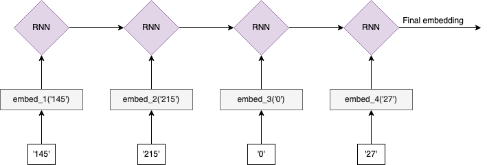
The key question is: what is meant by similar PII? There is not a single answer, and there are trade-offs among the strategies. For example, let's consider the task of learning embeddings for IP addresses. We might note that there is inherent structure to IPv4 values themselves (e.g., 145.215.0.27). The various octets give information about the type and location of the IP address. A simple strategy might be to split this value into the four octets (['145', '215', '0', '27']) and learn a separate embedding for each possible value in each position. However, there's additional structure in this data since it is increasingly specific when reading octets from left to right. For example, 123.210.54.90 is more similar to 123.20.15.22 (only first octets match) than it is to 95.210.54.90 (all but first octets match) even though the second one has more exact matches. This is because it is only relevant that the second octets match if the first octets also match, otherwise it's just a coincidence. We can try to exploit this conditional structure by feeding this left-to-right sequence of octet embeddings into an RNN model to produce a final IP embedding:

What is our training objective? One option might be optimizing the embeddings/RNN parameters to directly predict fraud, assuming we can associate fraud labels with each IP address. In this setup, “similar” would mean “similar fraud risk”. For a new IP address we would then split the octets, look up the learned embeddings of each, and then feed the sequence into the learned RNN model to produce a final IP address embedding for use in a downstream task.

There are similarities with the enrichment strategy. We should first note that different IP blocks (i.e., a set of IP addresses with shared leading octets) are allocated to particular Internet Service Providers (ISPs). Since the metadata essentially describes ISPs, this means that the octets have a strong correlation with the metadata and grouping by shared octets will therefore have similar outcomes as grouping by shared metadata.

There are important differences with the enrichment strategy, however. When grouping by enrichments, metadata of two IPs either matches or it does not. With embeddings, we can encode degree of similarity via distance in the embedding space. It could be, for example, that some subset of IPs within a single Internet Service Provider all belong to a university or large organization and have a similar risk profile distinct from the broader group. Since our embeddings are learnable, we have some flexibility in determining how things should be grouped together rather than relying on the hard boundaries of metadata.

Another difference is that we can in principle memorize that particular PII is fraud or legitimate since we ultimately learn the risk of a particular position in the embedding space. However, this “PII memorization” is in tension with our goal of making generalizable risk measures. For our method to be generalizable we want our predictions to be smooth across the embedding space. If this mapping is not smooth, then moving a small distance from a training sample will result in unstable predictions. We have some ability to control this trade-off by e.g., changing the dimensionality of our embedding space or the power of the model that consumes the embeddings, which in effect control how coarsely we group PII together.

A different embedding strategy makes an alternative trade-off. Instead of splitting our IP address based on octet and relying on the structure in the data, let's instead formulate our problem this way:

1. Treat each IP address as a “word” in a vocabulary
2. Create “sentences” by constructing IP address histories associated with a single entity, such as an account

Our data might look something like:

user_1 = ['125.65.19.102', '125.65.19.107', '125.65.39.5']
user_2 = ['78.123.98.12', '204.15.209.5', '40.23.2.17']

We can then apply a word2vec training strategy, in which we learn embeddings by using the surrounding IP addresses in the “sentence” to predict the target IP address (see my article on Noise Contrastive Estimation). In this setup, we define “similar” as “co-occuring in the same user history” and learn a separate embedding for each IP address. The drawback is that we'll need a lot of data and we will only have embeddings for IP addresses that we've seen before. Here we have high specificity since each IP address has its own embedding, but no generalization since we have no embedding for a new IP address that was not observed during training.

With embeddings we are able to make different trade-off decisions by both controlling the design of our modeling approach and the parameters of the model, like the dimensionality of the embedding space. [Note: we can, of course, use enrichment data in our embedding problem if available, which gives us further options.]

Graphs

An alternative way of framing the problem is by explicitly modeling the relationships between entities based on the knowledge that they used the same PII. For example, two accounts can be said to be “related” if they use the same IP address, credit card…etc. We can use graph structures to encode these relationships in a variety of ways. One option is to have “user” node-types that connect to PII data node-types, as below.

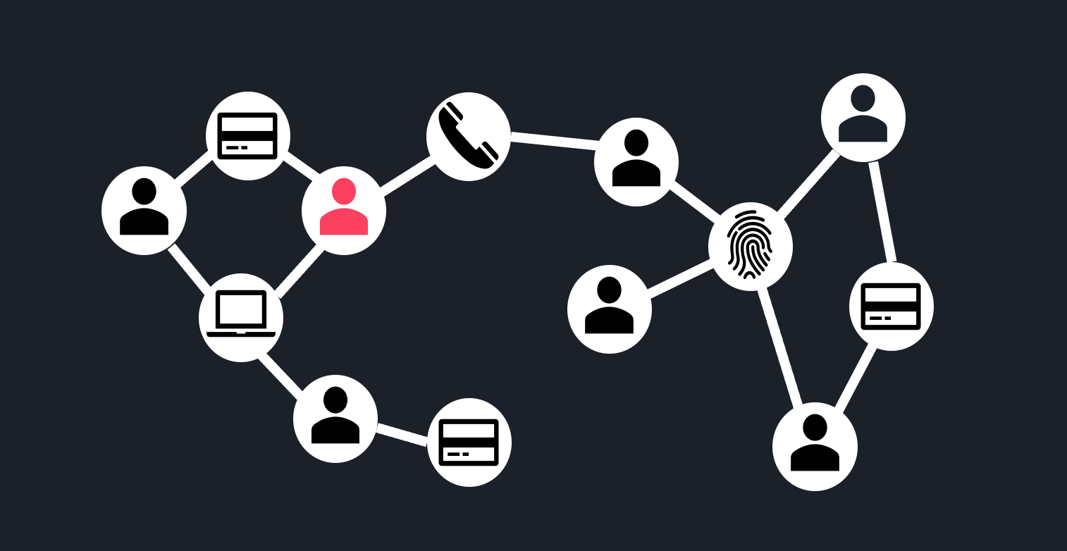
The key difference with other methods is that this approach breaks the assumption that the observations are independent from one another. This assumption of independence is foundational to most ML methods. Here we are saying something different: the fraud risk of a user is not independent of the fraud risk of other users, but in fact is dependent on related users based on shared PII data. This makes intuitive sense: the risk of an IP address is not fully determined by the Internet Service Provider or its metadata, but also depends on the history of entities that have used this IP address.

This approach encodes the notion of “guilt by association”. With this concept we can then infer that the user sharing a credit card with a know fraud actor, marked in red above, is high risk. Note that this does not rely on metadata or an understanding of what “similar PII” means. Instead, PII is used to simply relate entities to one another. The drawback to this approach, of course, is that it does not generalize to unseen PII data. Our graph will not help tomorrow if we get a new account that is using a previously unseen credit card.

Conclusions

In summary:

1. Enrichments give us strong generalization ability, but we lose the ability to distinguish specific PII data elements since our data is broadly coarsened together to facilitate statistical learning
2. Embeddings give us more control to make different trade-off decisions by changing our modeling approach (and even the hyperparameters of our methods)
3. Graphs can be used to directly model relationships based on specific PII, but these do not help generalize to unseen PII data

A strong system will use a balance of the above approaches so that we can both generalize to unseen PII and leverage our knowledge of what we observed in the past with particular PII data. There will be much more to say about the use of graphs in a future post, but before getting to this, we will first dive into the pervasive problem of noisy labels in Part 3.