Noise Contrastive Estimation

Introduction

I have recently worked to understand Noise Contrastive Estimation (NCE), and it was a tough journey. This post is meant to make it easier for other people by being less formal, and working through the particulars of implementation. Before digging into the details of how it works, let's first talk about the problem it sets out to solve.

Background

Let's say you want to learn vector embeddings of words to help with Natural Language tasks. The famous word2vec approach does something clever:

1. Start with a sentence: “the quick brown fox jumps”
2. Use a sliding window across the sentence to create (context, target) pairs, where the target is the center word and the context is the surrounding words:

• ([the, brown], quick)
• ([quick, fox], brown)
• ([brown, jumps], fox)

3. Use a lookup embedding layer to convert the context words into vectors, and average them to get a single input vector that represents the full context.
4. Using the context vector as input into a fully connected Neural Network layer with a Softmax transformation. This results in a probability for every word in your entire vocabulary for being the correct target given the current context.
5. Minimize the cross-entropy loss where label = 1 for the correct target word, and label = 0 for all other words.

By doing this, the network learns the statistics of how often words occur together in sentences. Since the weights of the embedding lookup table are learnable, it tends to put similar words closer together in the embedding space than dissimilar words. Cool.

But let's think about the computation in Step 4 above. Your network's dense layer has a weight matrix of size (embedding_dim, vocab_dim), which transforms the context embedding into numbers that help you predict the probability of each vocabulary word. This requires two steps: 1) get a value for each word from the output of the dense layer (we'll call the values \( z_i \), where \( i \) indexes a particular word in the vocabulary), and then 2) turn those values into probabilities by using a Softmax transformation:

\[ p( \mathbf{z} )_i = \frac { e^{z_i} } { \sum_{j=1}^{\left\lvert V \right\rvert } e^{ z_j } } \]

Notice that the denominator requires a sum over the entire vocabulary size \( \left\lvert V \right\rvert \). If you have a huge vocabulary size, then it becomes expensive and slow to normalize each and every training example by summing over the outputs of every vocabulary word.

In Step 5, we calculate the cross-entropy loss:

\[ L = - \sum_{j}^{\left\lvert V \right\rvert } y_j log(p_j) = - log(p_{target}). \]

Even though the loss function is expressed as a sum over the entire vocabulary, the only term that is non-zero is where the label \( y_j = 1 \); i.e. the term corresponding to the actual target word. The problem is that every \( p_i \) term divides by the same denominator, which itself is a sum over the entire vocabulary. This makes our loss function depend on every output in the network, when means every network parameter will have a non-zero gradient and therefore needs updating for every training example.

Negative Sampling

One idea to solve this problem is: instead of summing over the probabilities of every incorrect vocabulary word in the denominator, just pick a few. These chosen non-target words are called Negative Samples. So: follow the same steps as above, but in Step 4, only make predictions for the target word and a random sample of the other words, and pretend that represents the entire vocabulary.

This will clearly not given the right normalization since you're not summing over the vast majority of the vocabulary, but it's an approximation that turns out to work well. It has the added advantage that you don't need to update the weights for every vocabulary word, which can be millions of parameters, but instead only the weights for the target word and the negative samples. Since this probability is normalized using just the target word and a few negative samples instead of the entire vocabulary, there's many fewer variables involved. The number of gradients/updates therefore goes from \( \left\lvert embed \right\rvert * \left\lvert V \right\rvert \) to \( \left\lvert embed \right\rvert * (\left\lvert samples \right\rvert + 1) \). This makes sense intuitively as well. Should we really use/update the parameters for the word “zebra” for every slice of every sentence available?

Noise Contrastive Estimation

NCE is very similar to Negative Sampling in implementation, but it adds some theoretical teeth. Let's first discuss how they frame the problem and then go through the tweaks to the implementation.

Learning by Comparison

In Negative Sampling, we labeled the true target word with 1, and random samples of the incorrect target words with 0s. This is sort of like training a model to predict, “Which of these is real, and which is noise?” NCE uses a Logistic Regression (LogReg) model to answer this question directly.

Recall that LogReg models the log-odds ratio that the input came from one class instead of another: \[ logit = log(\frac{p(1)}{p(2)}) = log(\frac{p(1)}{1-p(1)}).\] We want the log-odds that a class came from the true word-distribution \(P\) instead of a noise distribution \(Q\): \[ logit = log(\frac{P}{Q}) = log(P) - log(Q).\]

This compares the data distribution, which we're trying to learn, to a reference noise distribution–hence the name Noise Contrastive Estimation. We don't know the real distribution, \( P\), but we're free to specify \( Q \) to be whatever we want. The \( Q \) distribution is what we use to generate our Negative Samples. For instance, maybe we sample all vocabulary words with equal probability, or in a way that takes into account how rare a word is in the training data. The point is: it's up to us, and that makes calculating the \( log(Q) \) part straight-forward.

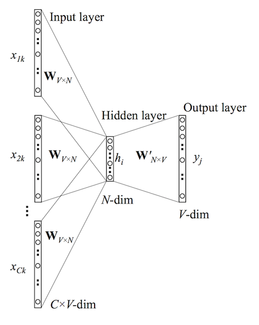
To be super-clear, I think it's worth looking one more time at the word2vec network and thinking about how \(Q \) is used:

We use a context vector as input into our dense layer. But instead of calculating the outputs of every single word in the vocabulary, we do the following: Randomly sample words from a distribution we've specified: \(Q\). Then only calculate the network output values for the true target word and for the words we randomly sampled from our noise distribution. If we pulled 5 random samples, then we would only evaluate the network for 6 outputs (samples + target), and ignore the rest of the vocabulary.

Now, since we define the Noise Distribution that determines how we pull the Negative Samples, we can analytically calculate any particular word's probability according to this distribution, \( Q \). For instance, if we define “word-1” to have probability 10% and “word-2” with probability 90%, and we happen to pull a sample of “word-1”, then \( Q = 0.10\); it's just a reference to the distribution we defined. So we can get the \( log(Q) \) part in \( logit = log(\frac{P}{Q}) = log(P) - log(Q) \). What about \( P \)?

That's what we use our neural network for–to predict \( P \) given a context. We then use the network output and the analytically calculated \( Q \) to calculate \( logit = log(\frac{P}{Q}) = log(P) - log(Q)\). The network is trained by treating this as a normal Logistic Regression task where the target word is labeled with 1 and the negative samples are all labeled with 0.

Using this framework, we transformed the unsupervised task of learning the data's probability distribution \( P \) into a supervised LogReg problem, in which we invent the labels by merely indicating if a word is the true target or came from the noise distribution. By learning a model to tell the difference between the real thing and a thing we invented, \(Q \), it learns to understand the real thing. Pretty clever framework.

Implementation

Now that we understand we want to create a Logistic Regression model to predict the log-odds of being real vs from the noise distribution, let's describe how we need to change the word2vec implementation. Steps 1-3 are identical: we create the same (context, target) pairs, and average the embeddings of the context words to get a context vector.

• In Step 4, you do the same thing as in Negative Sampling: use the context embedding vector as input to the neural network, and then gather the output for the target word and a random sample of \( k \) negative samples from the noise distribution, \( Q \).
• For the network output of each of the selected words, \( z_i \), subtract \( log(Q) \): \[ y_i = z_i - log(Q(i)) \]
• Instead of a Softmax transformation, apply a sigmoid transformation, as in Logistic Regression. This is because we're trying to model the logit, or the log-odds: \[ \hat{p_i} = \sigma(y_i) = \frac{1}{1+e^{-y_i}} \]
• Label the correct target word with label=1 and the negative samples with label=0.
• Use these as training samples for a Logistic Regression, and minimize the Binary Cross Entropy Loss: \[ BCE = \frac{1}{N} \sum_i^N l_i log(\hat{p_i}) + (1-l_i) log(1 - \hat{p_i})\]
  • Here, \( N = k + 1 \) (number of negative samples plus the target word), \( l_i \) are the labels for if it's the target or a negative sample, and \( \hat{p_i} \) are the outputs of the sigmoid as defined above.

The only real implementation difference from Negative Sampling is that there's a correction added, which takes into account the probability that the word is sampled, and then it's cast as a Logistic Regression/binary classification task. By using our network to output \(P \) and minimizing the Binary Cross Entropy, our network learns \(P\).

Note: In this form, the network is technically not outputting normalized values–there's nothing inherently enforcing that the outputs sum to 1. Adding explicit normalization would require summing over the entire vocabulary, which defeats the entire purpose. The original paper suggests that the normalization constants for each input context be a learnable parameter, and this is shown to work. However, it's been shown that, surprisingly, just assuming the network outputs normalized values gives equivalent performance, and the network learns to mostly self-normalize, since this is the optimal solution.

Conclusion

Noise Contrastive Estimation is a way of learning a data distribution by comparing it against a noise distribution, which we define. This allows us to cast an unsupervised problem as a supervised logistic regression problem. It's implementation is similar to Negative Sampling, which is an approximation mechanism that was invented to reduce the computational cost of normalizing network outputs by summing over the entire vocabulary. The primary difference in implementation between NCE and Negative Sampling is that in NCE, the probability that a sample came from the noise distribution is explicitly accounted for and the problem is cast as a formal estimate of the log-odds ratio that a particular sample came from the real data distribution instead of the noise distribution.

Resources

• The original NCE paper
• The adaptation of NCE for learning word embeddings
• A useful set of notes summarizing the theory of NCE
• TensorFlow's Candidate Sampling reference, which summarizes the similarities and differences among different sampling techniques, like Negative Sampling and NCE
• A deeper dive into word2vec. Part 1 has the basics and Part 2 concerns Negative Sampling and other improvements.