Noisy labels can wreak havoc

Introduction

Part 1 made a case for the use of ML in fraud detection applications and Part 2 dove into the challenges of modeling with Personally Identifiable Information (PII). In this post, I want to explore another challenge pervasive in fraud modeling: label noise. While some degree of label noise is common in many industrial applications, the problem is particularly pathological in the case of fraud detection systems and can lead to counter-intuitive results. If nothing else, it's a good story that demonstrates what people mean by a gap between academic ML and real-life applications.

Where noisy labels come from

Most fraud systems have the very sensible policy of innocent until proven guilty. In practice, there is probably a table somewhere that contains a list of all the confirmed fraud entities, and anything not on that list is therefore legitimate. Simplifying a bit, our labeling policy is something like “if it's in this fraud list then the label is 1, or if it's not in this list then the label is 0”.

Consider how labels change through time in the ideal case. Unless a bad actor is detected exactly at the point of account creation, they will have a legitimate label of 0 at some point. The fraud status will be identified in the future, and then the label will be changed from 0 to 1. In the period before we flip the label, we can say the entity had a “noisy label”. In other words, all bad actors have the wrong label at some time and the question is “for how long?" For a legitimate actor, they will start with and maintain the proper label. We can mistakenly mark legitimate actors as fraud, and this is also a source of label noise, but we assume here that these mistakes are rare compared to the amount of undetected fraud.

This is considered class-conditional label noise because the probability that our ground truth label is wrong (i.e., the “noise rate”) is different if the true class is “fraud” than if the true class is “legitimate”. Furthermore, we expect this noise rate to change with time since we will correct labels for bad actors as our detection systems identify them. In particular, the noise rate for labels of bad actors is initially 100%, and then decays according to the “time-to-detection” of our system. For example, if we identify 80% of the fraud within 7 days, the noise rate is reduced to 20% at that point.

Defining the training set

Let's consider the task of defining a training, validation and test dataset for the purposes of building an ML model. In general, we pull a snapshot of accounts at any given time and assign their labels based on the policy above. With class-conditional label noise, this setup implies that those with label==1 are accurately labeled, but those with label==0 consists of two populations: “truly legitimate” and “undetected fraud”. Assuming we don't want to train our model with incorrectly labeled examples, we face an immediate challenge: which of the label==0 population are reliably legitimate? The flip-side to this question is: which of the label==0 population are undetected fraud? However, if we had a good method for answering that question, we would have no need for a model in the first place!

In practice, I have seen three methods to make progress on this question.

1. Only use old data for training. This waits for our normal detection systems to identify fraud and therefore removes noise in the label==0 population. The appropriate time to wait depends on the detection systems and the target noise rate. The draw back is that if you only train on old data, your model may not learn the latest fraud patterns. However, one trick to get around this is to directly exploit the class-conditional nature and use different time periods for your label==0 and label==1 populations. Specifically, allow your label==1 population to span the full time range since these labels are reliable, but restrict the label==0 population to be old to reduce noise from undetected fraud. Using the most recent fraud labels is desirable because it gets the latest fraud patterns, and delaying the label==0 population is typically not a problem because legitimate actors have relatively stable behavior and therefore the model does not need the most recent legitimate data for learning.
2. Use a heuristic to define “reliably legitimate” that will select a reliable subset of your label==0 population. This might be, for example, that the entity has paid the business >$10. Depending on the business, this might ultimately reduce to something similar to tactic 1, since it may take considerable time for a new account to accrue billing and pay. This example would not be effective if bad actors are willing to make small purchases as a tactic to avoid detection, and this will in turn depend on the economics of the situation.
3. Filter based on an upstream model score with known performance characteristics. For example, if there's an “account registration” model and it's known that the fraud rate is less than 1% for the population where the score is less than 0.05, then we could filter the label==0 accounts to this sub-population. This establishes a dependency on this upstream model. Our filtering will only be as good as that model and we could bias our population in ways that are hard to understand.

In all cases, we must be careful with how these methods affect the resulting populations and therefore our results. For example, each of these methods is likely to change observed fraud rate compared to the baseline truth with no label noise. This will skew metrics that depend on relative population sizes, like precision, and we will therefore need to depend on metrics that are robust to population size differences, like Receiver Operating Characteristic (ROC) curves.

Model selection with label noise

Next, consider a situation with a population of undetected fraud in the validation/test sets. Let's say we have two models we want to compare: “Prod” (production) and “Research”. For the sake of illustration, let's say that the Research model identifies all the uncaught fraud of the Prod model in addition to all the correctly identified fraud, meaning the Research model is strictly better. We get scores on our test data, evaluate performance and see…the Prod model out-performs the Research model?!?

Why do we get exactly the wrong result? Consider how an uncaught fraud is evaluated. By definition of being “uncaught”, it has label==0. The Prod model says it is legitimate and therefore it is evaluated as the model correctly ignoring the account (a “True Negative”). However, the Research model says it is fraud, and is therefore evaluated as incorrectly marking a good account as fraud (a “False Positive”). The Research model is correct, but our ground truth label is wrong and so we count it as a False Positive instead of a True Positive. Even though our Research model is better than the Prod model, the existence of label noise results in us penalizing the metrics of models that fix the noise.

In other words, the better our model is at correcting the noise, the worse it will appear on the metrics. This makes it very difficult to tell whether a new research model is better or worse than production since both can cause metrics to drop. This requires a different mental muscle than data scientists are used to exercising, as we've been conditioned through e.g., reading papers and Kaggle exercises, that we evaluate models on our test dataset and the best metrics correspond to the best models. This paradigm works with clean data, but the situation is more nuanced in the presence of label noise.

Causal impact of production

Why is it that the production model gets the consistent benefit of the noise whereas the research model gets penalized? This is due to the causal impact our production systems have on our labels. If our detection systems are responsible for flagging high-risk accounts for human review, then the fraud that our systems miss will not get reviewed and therefore have the wrong label for a longer period of time. In other words, our system naturally perpetuates the mistakes of our models. Until we correct this noise, it will look like a good decision on the metrics. The production models will therefore have an unfair advantage in the presence of noise when compared to non-production models, where “non-production” means models that do not affect fraud outcomes.

We see that our ground truth labels are not ordained by God, but are rather the result of an imperfect feedback loop. To bootstrap reliable labels we are presented with a “chicken and the egg” problem since poor labels cause poor models, which in turn drive poor labels. How do we escape? There are no silver bullets. The first step is being aware of this dynamic and allowing it to permeate your understanding so that the right questions are asked and you're not led to the wrong answer by blindly trusting the ground truth. That said, we can look for mechanisms that help us escape the feedback loop. For example, in the case of a research model, we can have its supposed “false positives” investigated to see how many of them are actually true positives with the wrong label. This imbues the research model with the same causal advantage as production.

Production models can also have biased false positive metrics. This is because we often assign a fraud label whenever we take a fraud enforcement action, and this will ideally occur before we actually observed fraud. We therefore have the risk that we take a fraud action on a legitimate account and never get the feedback signal that we were incorrect. One technique for measuring these false positives is to allow some fraction of our high-risk entities to pass our systems unenforced and verify that they actually turn out to be fraud. This incurs some cost, of course, but it's the only reliable way to get accurate ground truth for fraud.

Choosing a decision threshold

The task of choosing a decision threshold on a model is also highly sensitive to the presence of class-conditional label noise and this can significantly limit our fraud detection ability. As an example, let's say our goal is to find the threshold that gives us a 1% False Positive Rate (FPR), as the business is unwilling to accept mistakes on legitimate customers above this level. For simplicity, let a 1% FPR correspond to a budget of 2 false positives in the image below. We therefore start drawing a threshold at the highest model score and move from right to left, counting the number of false positives. Once we reach two, we stop. Let the red indicate fraud, dark blue indicate legitimate, and light blue indicate uncaught fraud with a (noisy) legitimate label.

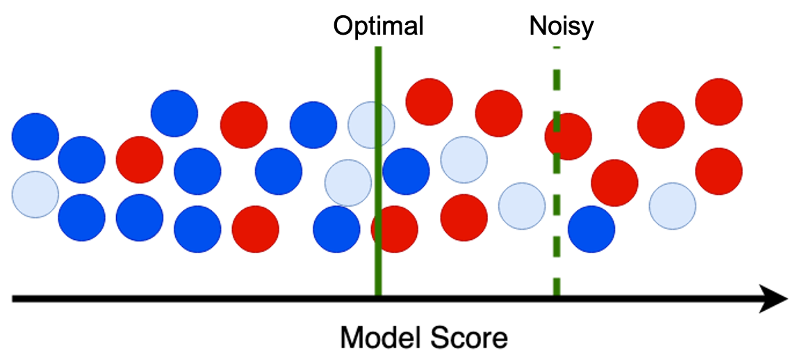
When the uncaught fraud have the wrong label, they are counted as false positives and we therefore stop at the “Noisy” line where we seem to have 2 false positives and 5 captured fraud. If we corrected the noise and re-colored the light blue as red fraud, then we would only count the dark blue as false positives and therefore stop at the “Optimal” line. Not only would our fraud capture metrics improve because of the 3 corrected noise, but we also gain detection of the 4 additional fraud that are below the “Noisy” threshold and above the “Optimal” threshold.

In other words, the presence of class-conditional label noise causes an overestimation of the false positive rate and therefore systematically biases our thresholding process to choose scores that are higher than we desire. Since a good model has a steep ROC curve, meaning that the fraud capture changes abruptly with small changes in FPR, this can have severe consequences in how much fraud we capture. In one case I've observed that around 5% of uncaught fraud can cause a 25% reduction in fraud capture as a result of setting the wrong decision threshold.

To combat this effect, we of course need clean data. For example, we can build a “Gold Standard” validation set where we've taken great effort to remove noise by manually investigating supposed false positives. Or, instead of doing FPR-targeting on a validation set from the newest data (as the typical “out-of-time” validation strategy prescribes), we can run this FPR-targeting process on old data prior to the training period. If we know that noise is reduced with time, this will give us more reliable estimates of FPR because this metric only relies on the label==0 population and therefore is only sensitive to noise there. This will not, however, give you a reliable estimate of your true positive rate, since the fraud populations can be quite different across time and in general models tend to perform better at finding older fraud than newer.

Conclusion

Here we have discussed a number of nuances that result from having noise in the labels. Because of our “innocent until proven guilty” setup that assigns label==0 to everything by default, we get a number of problems when trying to apply standard ML techniques. Further, since our fraud labels are identified by the feedback loop of our production systems, the metrics are biased in favor of production models, and this makes it difficult to break out of the cycle.

The aim of these examples is to prime your brain to be on the lookout for these effects. To avoid falling into traps we need to be deliberate about our goals and carefully consider how the existence of noise may bias the results. By starting with these questions, we can hopefully find a reliable solution. For example, if our goal is FPR-targeting, we can ignore the standard advice of using “out-of-time validation” because we know our goal is sensitive to noise in the label==0 population, and that the newest data has the highest noise level. Or, when developing a new research model, we can anticipate that our metrics may appear to be worse even though our model is better, and therefore include a process into our research plan that helps us address this potential source of error. I would advocate that any research proposal in a fraud setting would have a section dedicated to exploring the impact of label noise and methods to address it.

To wrap up this blog series on Fraud ML, I will next dive into the use of graphs and Graph ML in Part 4.