Overview of GANs - Part II

Introduction

In Part I of this series, the original GAN paper was presented. Although being clever and giving state of the art results at the time, much has been improved upon since. In this post I’ll talk about the contributions from the Deep Convolutional-GAN (DCGAN) paper.

Motivation

Part I concluded with an enumeration of some problems with GAN. Chief among them was training stability. DCGAN makes significant contributions to this problem by giving specific network architecture recommendations.

These recommendations are targeted toward the computer vision domain, which has been one of the most successful application areas of deep learning. Specifically, the use of convolutional layers.

DC GAN

Let’s jump in to the architecture details. I’ll assume basic familiarity with convolutional layers. If you need this background, check out this post. The recommended changes come directly from advances in the computer vision literature.

1. Replace pooling layers with strided convolutions. Historically, CNNs used pooling layers to reduce dimensions. For instance, a 2x2 max pooling layer would take a 2x2 array of pixels and map to one number, which is the max among them. A strided convolution can decrease the dimension by jumping multiple pixels between convolutions instead of sliding the kernel one-by-one. Similarly, it can increase dimension by adding empty pixels between the real ones, called fractional-strided convolution. This is a great resource for learning more about the details of strided convolutions, but the point is that this allows the network to learn it’s own spatial down- or up-sampling.
2. Remove fully connected layers and directly connect the output to the convolutional layers.
3. Batch normalization. This re-scales the input at each layer to have a mean of zero and unit variance. It’s claimed this greatly helps the onset of model learning and helps avoid mode collapse. Batch norm was not applied, however, to the Generator output layer or the Discriminator input layer (i.e. the image layers), as this led to instability.
4. ReLU activation in the Generator (except output layer which uses tanh), and leaky ReLU for Discriminator. It’s claimed this helps learn to cover the color space more quickly.

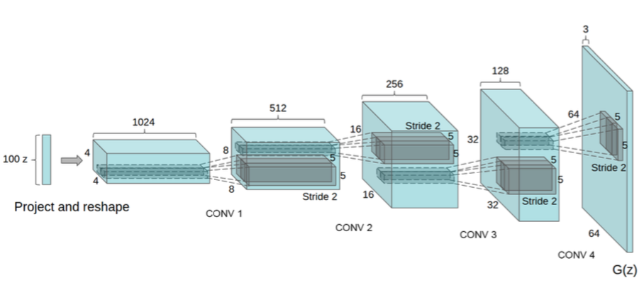
The Generator is shown above, and the Discriminator is essentially a mirror image. The 100-D noise input is fully connected to the high level convolutional features. This layer then uses fractional-striding to double the size of the filters, but creates half the number. This process of doubling in size, halving the number is repeated until 128 filters of size 32x32 are created. This is then upscaled to a 64x64 image with 3 layers, representing the three color channels.

Results

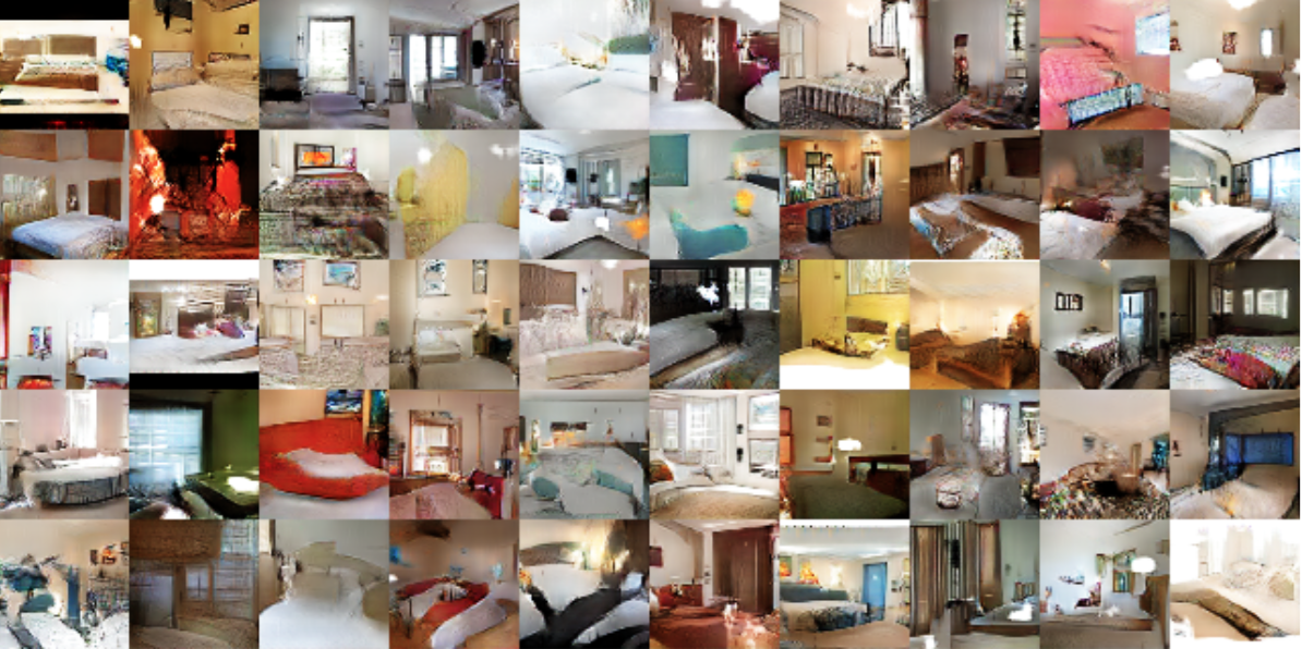
Here are some generated images of bedrooms after 5 epochs of training on the LSUN bedrooms dataset. Pretty cool.

To further demonstrate that the Generator was learning meaningful, high level features, they conducted an experiment with “image arithmetic”.

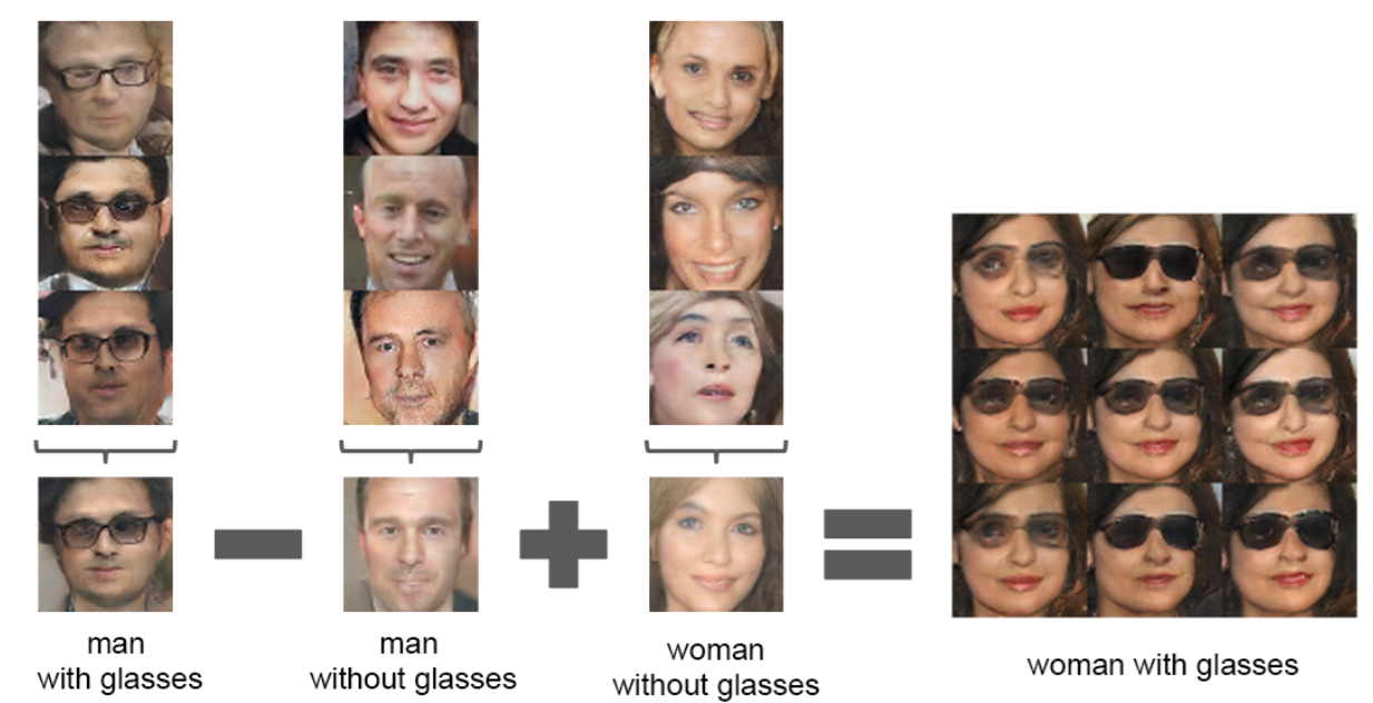
Here they have taken a man with glasses, subtracted out “man”-ness, added “female”-ness, and the results are a female with glasses. This suggests there are dedicated parts of the Generator that control the presence of glasses and the gender. This was accomplished by doing these arithmetic operations on the Generator noise input. So, you take the z-input vector for man with glasses, subtract the z-input vector for man with no glasses…etc. The resultant vector is then fed into the Generator to come up with the desired image. Multiple similar images were created by adding small, random changes to the input vector.

A more systematic example of this was given by interpolating in the direction between faces that looked right and left. So you start with a vector representing right-looking faces and slowly move it in the direction of left-looking faces. This is the result:

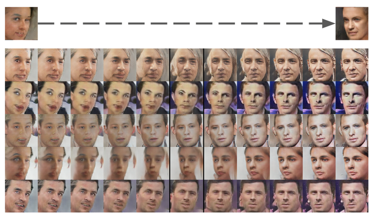
This shows that by walking in the latent/noise-space z, you can have systematic control over features in the generated samples!

Finally, they also demonstrated the quality of the Discriminator by removing the real/fake classifier and feeding the convolutional features into a new classifier — i.e. the Discriminator was a feature extractor. If it’s true that useful, general features were learned, then it should be straight-forward to train a classifier by using these features. Using CIFAR-10, which has 10 different image classes, it had competitive accuracy at 83%. Interestingly, the DCGAN was not trained on the CIFAR-10 dataset itself, but on Imagenet-1k. This shows that the model learned general, useful features since it gave great performance on a totally different dataset.

Problems

One of the remaining problems is that the representation is entangled. This means the useful aspects of the input vector z are entangled with the raw noise. If one could separate the “latent code” from the noise, then Generators would be more useful since you could control the output systematically and reliably without having to randomly walk the space. This problem and solution will be explored in the next section.